Just another Tensorflow beginner guide (Part2)
As we have tried some basic Tensorflow code and Tensorboard function in Part 1, here we are going to try some examples that is a bit more complicated
Study case 1: The MNIST dataset
Simple model - no hidden layer
You’ve probably already heard about MNIST dataset which contains lots of hand written digits pixel data.
I will not be able to give detailed explanations on how to use tensorflow to do a neural network to classify
those hand written digits but there are many good resource online. I will link a few below incase you haven’t
read them.
But anyway here is a working example I took from here that use TF to train a simple neural net to classify MNIST dataset, which by the end can reach 92% accuracy (without any hidden layer).
# example-2-simple-mnist.py
import tensorflow as tf
from datetime import datetime
import time

# reset everything to rerun in jupyter
tf.reset_default_graph()

# config
batch_size = 100
learning_rate = 0.5
training_epochs = 6
logs_path = './tmp/example-2/' + datetime.now().isoformat()

# load mnist data set
from tensorflow.examples.tutorials.mnist import input_data
mnist = input_data.read_data_sets('tmp/MNIST_data', one_hot=True)

# input images
with tf.name_scope('input'):
    # None -> batch size can be any size, 784 -> flattened mnist image
    x = tf.placeholder(tf.float32, shape=[None, 784], name="x-input")
    # target 10 output classes
    y_ = tf.placeholder(tf.float32, shape=[None, 10], name="y-input")

# model parameters will change during training so we use tf.Variable
with tf.name_scope("weights"):
    W = tf.Variable(tf.zeros([784, 10]))

# bias
with tf.name_scope("biases"):
    b = tf.Variable(tf.zeros([10]))

# implement model
with tf.name_scope("softmax"):
    # y is our prediction
    y = tf.nn.softmax(tf.matmul(x,W) + b)

# specify cost function
with tf.name_scope('cross_entropy'):
    # this is our cost
    cross_entropy = tf.reduce_mean(-tf.reduce_sum(y_ * tf.log(y), reduction_indices=[1]))

# specify optimizer
with tf.name_scope('train'):
    # optimizer is an "operation" which we can execute in a session
    train_op = tf.train.GradientDescentOptimizer(learning_rate).minimize(cross_entropy)

with tf.name_scope('accuracy'):
    # Accuracy
    correct_prediction = tf.equal(tf.argmax(y,1), tf.argmax(y_,1))
    accuracy = tf.reduce_mean(tf.cast(correct_prediction, tf.float32))

# create a summary for our cost and accuracy
train_cost_summary = tf.summary.scalar("train_cost", cross_entropy)
train_acc_summary = tf.summary.scalar("train_accuracy", accuracy)
test_cost_summary = tf.summary.scalar("test_cost", cross_entropy)
test_acc_summary = tf.summary.scalar("test_accuracy", accuracy)

# merge all summaries into a single "operation" which we can execute in a session
# summary_op = tf.summary.merge_all()

with tf.Session() as sess:
    # variables need to be initialized before we can use them
    sess.run(tf.initialize_all_variables())

    # create log writer object
    writer = tf.summary.FileWriter(logs_path, graph=tf.get_default_graph())

    # perform training cycles
    for epoch in range(training_epochs):

        # number of batches in one epoch
        batch_count = int(mnist.train.num_examples/batch_size)

        for i in range(batch_count):
            batch_x, batch_y = mnist.train.next_batch(batch_size)

            # perform the operations we defined earlier on batch
            _, train_cost, train_acc, _train_cost_summary, _train_acc_summary =
                sess.run([train_op, cross_entropy, accuracy, train_cost_summary, train_acc_summary],
                    feed_dict={x: batch_x, y_: batch_y})
            # write log
            writer.add_summary(_train_cost_summary, epoch * batch_count + i)
            writer.add_summary(_train_acc_summary, epoch * batch_count + i)

            if i % 100 == 0:
                # for log on test data:
                test_cost, test_acc, _test_cost_summary, _test_acc_summary =
                    sess.run([cross_entropy, accuracy, test_cost_summary, test_acc_summary],
                        feed_dict={x: mnist.test.images, y_: mnist.test.labels})
                # write log
                writer.add_summary(_test_cost_summary, epoch * batch_count + i)
                writer.add_summary(_test_acc_summary, epoch * batch_count + i)

                print('Epoch {0:3d}, Batch {1:3d} | Train Cost: {2:.2f} | Test Cost: {3:.2f} | Accuracy batch train: {4:.2f} | Accuracy test: {5:.2f}'
                    .format(epoch, i, train_cost, test_cost, train_acc, test_acc))

    print('Accuracy: {}'.format(accuracy.eval(feed_dict={x: mnist.test.images, y_: mnist.test.labels})))
    print('done')

# tensorboard --logdir=./tmp/example-2 --port=8002 --reload_interval=5
# You can run the following js code in broswer console to make tensooboard to do auto-refresh
# setInterval(function() {document.getElementById('reload-button').click()}, 5000);
Now after use python to run this python file, then start up tensooboard with $ tensooboard --logdir=./tmp/example-2 --port=8002 --reload_interval=5. Now you can
open in browser at http://localhost:8002/ then you should be able to see the
computation graph:
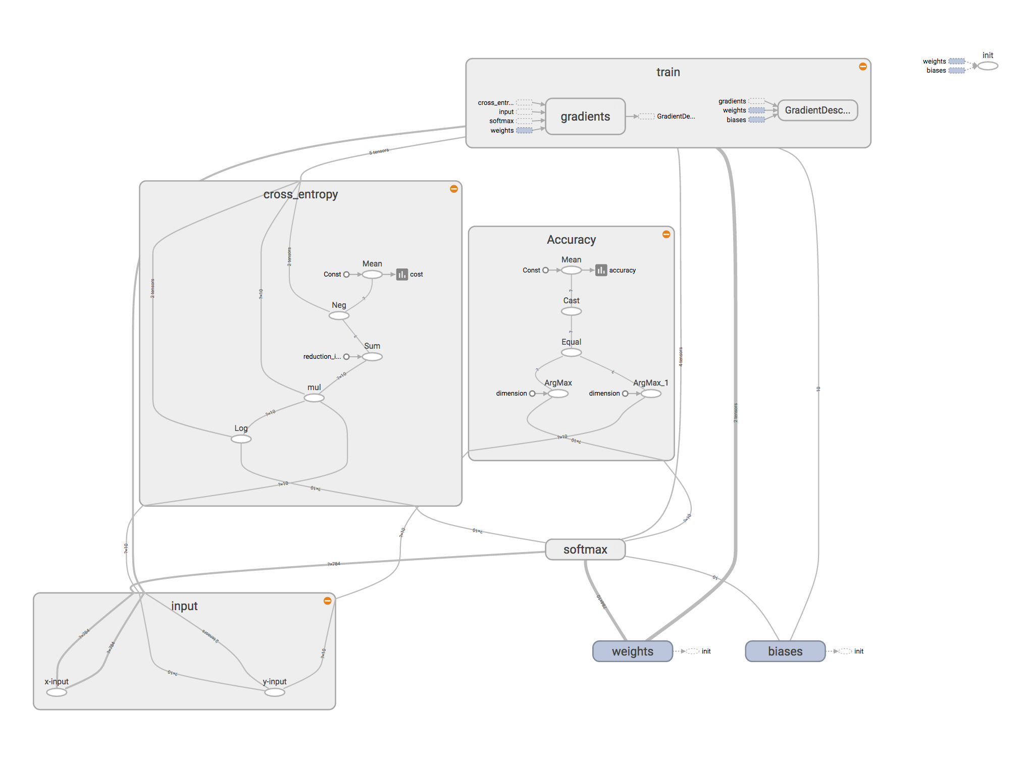 Tensorboard graph for simple MNIST model
Note that in the code we have used with tf.name_scope('xxx'): which is used to
group the graph components.
And on the scalar tab you can see some of those scalar summary such as the cost and
accuracy for training and testing, such as:
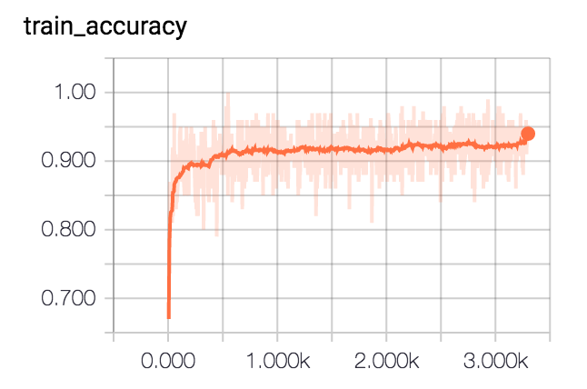 Tensorboard train accuracy summary for simple MNIST model
A bit more complex - Add one hidden layer
As we could see the 92% test accuracy of previous run is not too amazing, as we don’t have any hidden layer between the input and output vectors.
Thus we can simply add one hidden layer and see if it will help with increasing accuracy in someway. Theoretically it should help as long as the model is not overfitting.
We can add those changes in the code to add an extra layer:
- Add a parameter somewhere on the top part of code to define the hidden layer size - let’s try with 200
layer1_size = 200 - Add another weight
W1and biasb1as follow. Note that here we need to initialize those weights withtf.truncated_normal()method instead of initializing them as zeros like before. This is because (if I guess correctly) that with hidden layers existing, the feed forward and back propagation will not be able to contribute any value changes if those weights are initialized as zeros. (You might notice this if you forgot to update the initialization code)with tf.name_scope("weights"): W1 = tf.Variable(tf.truncated_normal([784, layer1_size], stddev=0.1)) W = tf.Variable(tf.truncated_normal([layer1_size, 10], stddev=1.0)) with tf.name_scope("biases"): b1 = tf.Variable(tf.zeros([layer1_size])) b = tf.Variable(tf.zeros([10])) - Then add the hidden layer as:
with tf.name_scope('hidden_layers'): y1 = tf.nn.relu(tf.matmul(x, W1) + b1) - Next update the softmax output layer to use hiddlen layer
y1, also usetf.nn.softmax_cross_entropy_with_logits()to calculate the cost:with tf.name_scope("softmax"): ylogits = tf.matmul(y1, W) + b y = tf.nn.softmax(ylogits) with tf.name_scope('cross_entropy'): cross_entropy = tf.nn.softmax_cross_entropy_with_logits(logits=ylogits, labels=y_) cross_entropy = tf.reduce_mean(cross_entropy) - Plus you might want to try a different optimizer:
  with tf.name_scope('train'):
      train_op = tf.train.AdamOptimizer().minimize(cross_entropy)
That should be it, no other change is needed for the rest of the code. And if you run this code with one hidden layer (200 nodes), you should get the test accuracy above 96% :)
For those who want to make it perform even better, I think this Tensorflow and deep learning without a PhD is a good place to digging the MNIST dataset deeper.
Study case 2: A simple sentiment analysis
We can now try a simple sentiment analysis using most of code above but this time the fun part is the data will be a bit more realistic and one needs to some simple natural language processing on the incoming raw data.
You can get some sample code and the train test data here. And our example here is pretty much a copy of the tutorial of this youtube channel. So I guess you can follow the video as well, it discuss much more info than what I will write here.
First step: raw data to feature vectors
Basically, the first thing we need to do is to parse the input text and change them into
vectors with digits so we could feed them into a neural network. There are many ways of
doing this, such as bag of words, word2vec and so on. We will just follow the video tutorial
and use a very simple bag of words model and the script doing is called create_sentiment_featuresets.py.
You can run command as below, or check the info here about nltk. (Also make sure the train and test csv file are in the same folder)
$ cd example-3
$ pip install nltk
$ python -m nltk.downloader punkt wordnet
$ python create_sentiment_featuresets.py
The create_sentiment_featuresets.py will dump the extracted feature vectors into
a file under folder tmp and called sentiment_set.pickle, which will be used to load those
train test input data in the very next step.
Second step: train a model
Then for the second step, one can simply use the one layer model we made above for MNIST data, just a few places on loading data needs to be updated.
Such as the data loading part is replaces as:
# example-3.py
...
train_x, train_y, test_x, test_y = pickle.load( open('tmp/sentiment_set.pickle', 'rb' ) )
train_x = train_x.toarray() # as we stored the data as sparse matrix, restore them back to numpy array
test_x = test_x.toarray()
...
And the session running loop is now looking like:
# example-3.py
...
with tf.Session() as sess:
    # variables need to be initialized before we can use them
    sess.run(tf.initialize_all_variables())

    # create log writer object
    writer = tf.summary.FileWriter(logs_path, graph=tf.get_default_graph())

    # perform training cycles
    for epoch in range(training_epochs):
        # number of batches in one epoch
        batch_count = int(len(train_x)/batch_size)
        i = 0
        for _b in range(batch_count):
            start = i
            end = i + batch_size
            batch_x = np.array(train_x[start:end])
            batch_y = np.array(train_y[start:end])

            # perform the operations we defined earlier on batch
            _, train_cost, train_acc, _train_cost_summary, _train_acc_summary = \
                sess.run([train_op, cross_entropy, accuracy, train_cost_summary, train_acc_summary],
                    feed_dict={x: batch_x, y_: batch_y})
            # write log
            writer.add_summary(_train_cost_summary, epoch * batch_count + _b)
            writer.add_summary(_train_acc_summary, epoch * batch_count + _b)

            if i % 100 == 0:
                # for log on test data:
                test_cost, test_acc, _test_cost_summary, _test_acc_summary = \
                    sess.run([cross_entropy, accuracy, test_cost_summary, test_acc_summary],
                        feed_dict={x: test_x, y_: test_y})
                # write log
                writer.add_summary(_test_cost_summary, epoch * batch_count + _b)
                writer.add_summary(_test_acc_summary, epoch * batch_count + _b)

                print('Epoch {0:3d}, Batch {1:3d} | Train Cost: {2:.2f} | Test Cost: {3:.2f} | Accuracy batch train: {4:.2f} | Accuracy test: {5:.2f}'
                    .format(epoch, i, train_cost, test_cost, train_acc, test_acc))
            i += batch_size
    print('Accuracy: {}'.format(accuracy.eval(feed_dict={x: test_x , y_: test_y})))
    print('done')
Now run this example-3.py and you should see output such as
...
Epoch   5, Batch 8300 | Train Cost: 0.33 | Test Cost: 0.73 | Accuracy batch train: 0.85 | Accuracy test: 0.65
Epoch   5, Batch 8400 | Train Cost: 0.28 | Test Cost: 0.73 | Accuracy batch train: 0.87 | Accuracy test: 0.65
Epoch   5, Batch 8500 | Train Cost: 0.15 | Test Cost: 0.73 | Accuracy batch train: 0.97 | Accuracy test: 0.65
Accuracy: 0.6538461446762085
Looks like after epoch 3 we start to getting into a overfitting situation where the train accuracy is very high and the test accuracy is relatively low.
Now you may use some of the common ideas on tackle this overfitting issue, just to name a few here:
- Get more data!!
- Train with a smaller neural network
- Early stopping
- Train many big nets on random subsets of the data and average their predictions.
- Train the big neural net with dropout in the hidden units.
- Train many different models - neural nets, SVMs, decision trees - and average their predictions.
- Data augmentation
- Add un-supervised pre-training
I will just try method 1 here, make the neural network smaller see what happens.
So for the parameter layer1_size let’s change it from 200 to 32:
...
Epoch   5, Batch 8300 | Train Cost: 0.52 | Test Cost: 0.62 | Accuracy batch train: 0.73 | Accuracy test: 0.66
Epoch   5, Batch 8400 | Train Cost: 0.41 | Test Cost: 0.62 | Accuracy batch train: 0.81 | Accuracy test: 0.66
Epoch   5, Batch 8500 | Train Cost: 0.35 | Test Cost: 0.62 | Accuracy batch train: 0.90 | Accuracy test: 0.66
Accuracy: 0.6622889041900635
Looks like the results got better. (However we might just got a bit lucky here and the model is initialized randomly so you might have a different result here)
Summary
Congratulations, now you have used Tensorflow and your own raw data to make a simple model that can predict the sentiment on a given input movie comment. Apparently it is not that precise yet but I think we now have a good ground work to develop it further, with some feature engineering (for example perhaps use bigrams as well) together with some methods mentioned above for overfitting.
Later on I would like to try to use google cloud to help us do the calculation, instead of running the calculation locally. It might not make much of a sense for this small example but when you once have some big data on hands, doing cloud computation might be one of the solution as your local laptop might not be powerful enough.
Useful learning materials
- Google codelab - Tensorflow and deep learning, without a Phd - very good examples on TF and deep learning and if you go for the convolutional networks you can reach accuracy of 99% on MNIST dataset
- pythonprogramming.net